How to do it...

1. Import libraries and dataset:

import numpy as np 
from sklearn.model_selection import train_test_split
import matplotlib.pyplot as plt
# We will be using make_circles from scikit-learn
from sklearn.datasets import make_circles

SEED = 2017

1. First, we need to create the training data:

# We create an inner and outer circle
X, y = make_circles(n_samples=400, factor=.3, noise=.05, random_state=2017)
outer = y == 0
inner = y == 1

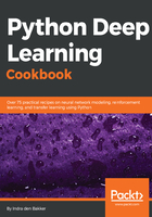
1. Let's plot the data to show the two classes:

plt.title("Two Circles")
plt.plot(X[outer, 0], X[outer, 1], "ro")
plt.plot(X[inner, 0], X[inner, 1], "bo")
plt.show()

1. We normalize the data to make sure the center of both circles is (1,1):

X = X+1

1. To determine the performance of our algorithm we split our data:

X_train, X_val, y_train, y_val = train_test_split(X, y, test_size=0.2, random_state=SEED)

1. A linear activation function won't work in this case, so we'll be using a sigmoid function:

def sigmoid(x):
 return 1 / (1 + np.exp(-x))

1. Next, we define the hyperparameters:

n_hidden = 50 # number of hidden units
n_epochs = 1000
learning_rate = 1

1. Initialize the weights and other variables:

# Initialise weights
weights_hidden = np.random.normal(0.0, size=(X_train.shape[1], n_hidden))
weights_output = np.random.normal(0.0, size=(n_hidden))

hist_loss = []
hist_accuracy = []

1. Run the single-layer neural network and output the statistics:

for e in range(n_epochs):
 del_w_hidden = np.zeros(weights_hidden.shape)
 del_w_output = np.zeros(weights_output.shape)

 # Loop through training data in batches of 1
 for x_, y_ in zip(X_train, y_train):
  # Forward computations
  hidden_input = np.dot(x_, weights_hidden)
  hidden_output = sigmoid(hidden_input)
  output = sigmoid(np.dot(hidden_output, weights_output))

  # Backward computations
  error = y_ - output
  output_error = error * output * (1 - output)
  hidden_error = np.dot(output_error, weights_output) * hidden_output 
                     * (1 - hidden_output)
  del_w_output += output_error * hidden_output
  del_w_hidden += hidden_error * x_[:, None]

 # Update weights
 weights_hidden += learning_rate * del_w_hidden / X_train.shape[0]
 weights_output += learning_rate * del_w_output / X_train.shape[0]

 # Print stats (validation loss and accuracy)
 if e % 100 == 0:
  hidden_output = sigmoid(np.dot(X_val, weights_hidden))
  out = sigmoid(np.dot(hidden_output, weights_output))
  loss = np.mean((out - y_val) ** 2)
  # Final prediction is based on a threshold of 0.5
  predictions = out > 0.5
  accuracy = np.mean(predictions == y_val)
  print("Epoch: ", '{:>4}'.format(e), 
        "; Validation loss: ", '{:>6}'.format(loss.round(4)), 
        "; Validation accuracy: ", '{:>6}'.format(accuracy.round(4)))

In the following screenshot, the output during training is shown: