Value, state, and optimality

You may remember our definition of the value of the state in Chapter 1, What is Reinforcement Learning?. This is a very important notion and the time has come to explore it further. This whole part of the book is built around the value and how to approximate it. We defined value as an expected total reward that is obtainable from the state. In a formal way, the value of the state is: , where is the local reward obtained at the step t of the episode.

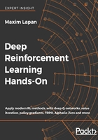
The total reward could be discounted or not; it's up to us how to define it. Value is always calculated in the respect of some policy that our agent follows. To illustrate, let's consider a very simple environment with three states:

1. The agent's initial state.
2. The final state that the agent is in after executing action "left" from the initial state. The reward obtained from this is 1.
3. The final state that the agent is in after action "down". The reward obtained from this is 2:
   

   Figure 1: An example of an environment's states transition with rewards

The environment is always deterministic: every action succeeds and we always start from state 1. Once we reach either state 2 or state 3, the episode ends. Now, the question is, what's the value of state 1? This question is meaningless without information about our agent's behavior or, in other words, its policy. Even in such a simple environment, our agent can have an infinite amount of behaviors, each of which will have its own value for state 1. Consider this example:

• Agent always goes left
• Agent always goes down
• Agent goes left with a probability of 0.5 and down with a probability of 0.5
• Agent goes left in 10% of cases and in 90% of cases executes the "down" action

To demonstrate how the value is calculated, let's do it for all the preceding policies:

• The value of state 1 in the case of the "always left" agent is 1.0 (every time it goes left, it obtains 1 and the episode ends)
• For the "always down" agent, the value of state 1 is 2.0
• For the 50% left/50% down agent, the value will be 1.0*0.5 + 2.0*0.5 = 1.5
• In the last case, the value will be 1.0*0.1 + 2.0*0.9 = 1.9

Now, another question: what's the optimal policy for this agent? The goal of RL is to get as much total reward as possible. For this one-step environment, the total reward is equal to the value of state 1, which, obviously, is at the maximum at policy 2 (always down).

Unfortunately, such simple environments with an obvious optimal policy are not that interesting in practice. For interesting environments, the optimal policy is much harder to formulate and it's even harder to prove their optimality. However, don't worry, we're moving toward the point when we'll be able to make computers learn the optimal behavior on their own.

From the preceding example, you may have a false impression that we should always take the action with the highest reward. In general, it's not that simple. To demonstrate this, let's extend our preceding environment with yet another state that is reachable from state 3. State 3 is no longer a terminal state, but a transition to state 4, with a bad reward of -20. Once we've chosen the "down" action in state 1, this bad reward is unavoidable, as from state 3 we have only one exit. So, it's a trap for the agent who has decided that "being greedy" is a good strategy.

Figure 2: The same environment, with an extra state added

With that addition, our values for state 1 will be calculated this way:

• "Always left" agent is the same: 1.0
• "Always down" agent gets: 2.0 + (-20) = -18
• "50%/50% agent": 0.5*1.0 + 0.5*(20 + (-20)) = -8.5
• "10%/90% agent": 0.1*1.0 + 0.9*(2.0 + (-20)) = -8

So, the best policy for this new environment is now policy number one: always go left.

We spent some time discussing naïve and trivial environments so that you realize the complexity of this optimality problem and can appreciate the results of Richard Bellman better. Richard was an American mathematician, who formulated and proved his famous "Bellman equation". We'll talk about it in the next section.